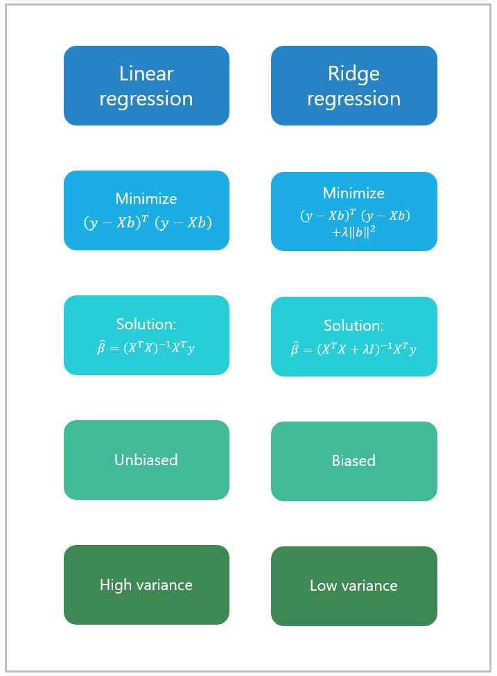
Ridge regression is a term used to refer to a linear regression model whose coefficients are estimated not by ordinary least squares (OLS), but by an estimator, called ridge estimator, that, albeit biased, has lower variance than the OLS estimator.
In certain cases, the mean squared error of the ridge estimator (which is the sum of its variance and the square of its bias) is smaller than that of the OLS estimator.
![]()
Ridge estimation is carried out on the linear regression
model![]() where:
where:
![]() is the
is the
![]() vector of observations of
the dependent variable;
vector of observations of
the dependent variable;
![]() is the
is the
![]() matrix of regressors (there are
matrix of regressors (there are
![]() regressors);
regressors);
![]() is the
is the
![]() vector of regression coefficients;
vector of regression coefficients;
![]() is the
is the
![]() vector of errors.
vector of errors.
Remember that the OLS estimator
![]() solves the minimization
problem
solves the minimization
problem![[eq2]](data:image/gif;base64,R0lGODlhAQABAIAAANvf7wAAACH5BAEAAAAALAAAAAABAAEAAAICRAEAOw==) where
where
![]() is the
is the
![]() -th
row of
-th
row of
![]() and
and
![]() and
and
![]() are
are
![]() column vectors.
column vectors.
When
![]() has full rank, the solution to
the OLS problem
is
has full rank, the solution to
the OLS problem
is![]()
The ridge estimator
![]() solves the slightly modified minimization
problemwhere
solves the slightly modified minimization
problemwhere
![]() is a positive constant.
is a positive constant.
Thus, in ridge estimation we add a penalty to the least squares criterion: we
minimize the sum of squared
residualsplus
the squared norm of of the vector of
coefficients
The ridge problem penalizes large regression coefficients, and the larger the
parameter
![]() is, the larger the penalty.
is, the larger the penalty.
We will discuss below how to choose the penalty parameter
![]() .
.
The solution to the minimization problem
is![]() where
where
![]() is the
is the
![]() identity matrix.
identity matrix.
The objective function to minimize can be
written in matrix form as
follows:The
first order condition for a minimum is that the gradient of
![]() with respect to
with respect to
![]() should be equal to
zero:
should be equal to
zero:![]() that
is,
that
is,![]() or
or![]() The
matrix
The
matrix![]() is
positive definite for
any
is
positive definite for
any
![]() because, for any
because, for any
![]() vector
vector
![]() ,
we
havewhere
the last inequality follows from the fact that even if
,
we
havewhere
the last inequality follows from the fact that even if
![]() is equal to
is equal to
![]() for every
for every
![]() ,
,
![]() is strictly positive for at least one
is strictly positive for at least one
![]() .
Therefore, the matrix has full
rank and it is invertible.
As a consequence, the first order condition is satisfied
by
.
Therefore, the matrix has full
rank and it is invertible.
As a consequence, the first order condition is satisfied
by![]() We
now need to check that this is indeed a global minimum. Note that the Hessian
matrix, that is, the matrix of second derivatives of
We
now need to check that this is indeed a global minimum. Note that the Hessian
matrix, that is, the matrix of second derivatives of
![]() ,
is
,
is![]() Thus,
the Hessian is positive definite (it is a positive multiple of a matrix that
we have just proved to be positive definite). Hence,
Thus,
the Hessian is positive definite (it is a positive multiple of a matrix that
we have just proved to be positive definite). Hence,
![]() is strictly convex in
is strictly convex in
![]() ,
which implies that
,
which implies that
![]() is a global minimum.
is a global minimum.
If you read the proof above, you will notice that, unlike in OLS estimation,
we do not need to assume that the design matrix
![]() is full-rank. Therefore, the ridge estimator exists also when
is full-rank. Therefore, the ridge estimator exists also when
![]() does not have full rank.
does not have full rank.
In this section we derive the bias and variance of the ridge estimator under
the commonly made assumption (e.g., in the
normal
linear regression model) that,
conditional
on
![]() ,
the errors of the regression have zero mean and constant variance
,
the errors of the regression have zero mean and constant variance
![]() and are
uncorrelated:where
and are
uncorrelated:where
![]() is a positive constant and
is a positive constant and
![]() is the
is the
![]() identity matrix.
identity matrix.
The conditional expected value of the ridge estimator
![]() is
is![]() which
is different from
which
is different from
![]() unless
unless
![]() (the OLS case).
(the OLS case).
The bias of the estimator
is![]()
We can write the ridge estimator
asTherefore,
![[eq22]](/images/ridge-regression__67.png) The
ridge estimator is unbiased, that
is,
The
ridge estimator is unbiased, that
is,![]() if
and only
if
if
and only
if![]() But
this is possible if only if
But
this is possible if only if
![]() ,
that is, if the ridge estimator coincides with the OLS estimator. where
,
that is, if the ridge estimator coincides with the OLS estimator. where
![]() is the
is the
![]() identity matrix. The bias
is
identity matrix. The bias
is
The covariance
matrix of the ridge estimator
is![]()
Remember that the OLS estimator
![]() has conditional
variance
has conditional
variance![]() We
can write the ridge estimator as a function of the OLS
estimator:Therefore,
We
can write the ridge estimator as a function of the OLS
estimator:Therefore,![[eq29]](/images/ridge-regression__78.png)
Importantly, the variance of the ridge estimator is always smaller than the variance of the OLS estimator.
More precisely, the difference between the covariance matrix of the OLS
estimator and that of the ridge estimator
![]() is
positive definite (remember from the lecture on the
Gauss-Markov
theorem that the covariance matrices of two estimators are compared by
checking whether their difference is positive definite).
is
positive definite (remember from the lecture on the
Gauss-Markov
theorem that the covariance matrices of two estimators are compared by
checking whether their difference is positive definite).
In order to make a comparison, the OLS
estimator must exist. As a consequence,
![]() must be full-rank. With this assumption in place, the conditional variance of
the OLS estimator
is
must be full-rank. With this assumption in place, the conditional variance of
the OLS estimator
is![]() Now,
define the
matrix
Now,
define the
matrix![]() which
is invertible. Then, we can rewrite the covariance matrix of the ridge
estimator as
follows:
which
is invertible. Then, we can rewrite the covariance matrix of the ridge
estimator as
follows:![[eq33]](/images/ridge-regression__83.png) The
difference between the two covariance matrices
is
The
difference between the two covariance matrices
is![[eq34]](/images/ridge-regression__84.png) If
If
![]() ,
the latter matrix is positive definite because for any
,
the latter matrix is positive definite because for any
![]() ,
we
have
,
we
have![]() andbecause
andbecause
![]() and its inverse are positive definite.
and its inverse are positive definite.
The mean squared error (MSE) of the ridge estimator
is equal to the trace of its
covariance matrix plus the squared norm of its bias (the so-called
bias-variance
decomposition):
The OLS estimator has zero bias, so its MSE
is
The difference between the two MSEs
is![[eq39]](/images/ridge-regression__92.png) where
we have used the fact that the sum of the traces of two matrices is equal to
the trace of their sum.
where
we have used the fact that the sum of the traces of two matrices is equal to
the trace of their sum.
We have a difference between two terms
(![]() and
and
![]() ).
We have already proved that the
matrix
).
We have already proved that the
matrix![]() is
positive definite. As a consequence, its trace (term
is
positive definite. As a consequence, its trace (term
![]() )
is strictly positive.
)
is strictly positive.
The square of the bias (term
![]() )
is also strictly positive. Therefore, the difference between
)
is also strictly positive. Therefore, the difference between
![]() and
and
![]() could
in principle be either positive or negative.
could
in principle be either positive or negative.
It is possible to prove (see Theobald 1974 and
Farebrother 1976) that whether the difference is
positive or negative depends on the penalty parameter
![]() ,
and it is always possible to find a value for
,
and it is always possible to find a value for
![]() such that the difference is positive.
such that the difference is positive.
Thus, there always exists a value of the penalty parameter such that the ridge estimator has lower mean squared error than the OLS estimator.
This result is very important from both a practical and a theoretical standpoint. Although, by the Gauss-Markov theorem, the OLS estimator has the lowest variance (and the lowest MSE) among the estimators that are unbiased, there exists a biased estimator (a ridge estimator) whose MSE is lower than that of OLS.
We have just proved that there exists a
![]() such that the ridge estimator is better (in the MSE sense) than the OLS one.
such that the ridge estimator is better (in the MSE sense) than the OLS one.
The question is: how do find the optimal
![]() ?
?
The most common way to find the best
![]() is by so-called leave-one-out cross-validation:
is by so-called leave-one-out cross-validation:
we choose a grid of
![]() possible values
possible values
![]() for the penalty parameter;
for the penalty parameter;
for
![]() ,
we exclude the
,
we exclude the
![]() -th
observation
-th
observation
![]() from the sample and we:
from the sample and we:
use the remaining
![]() observations to compute
observations to compute
![]() ridge estimates of
ridge estimates of
![]() ,
denoted by
,
denoted by
![]() ,
where the subscripts
,
where the subscripts
![]() indicate that the penalty parameter is set equal to
indicate that the penalty parameter is set equal to
![]() (
(![]() )
and the
)
and the
![]() -th
observation has been excluded;
-th
observation has been excluded;
compute
![]() out-of-sample predictions of the excluded
observation
out-of-sample predictions of the excluded
observation![]() for
for
![]() .
.
we compute the MSE of the
predictionsfor
![]() .
.
we choose as the optimal penalty parameter
![]() the one that minimizes the MSE of the
predictions:
the one that minimizes the MSE of the
predictions:![]()
In other words, we set
![]() equal to the value that generates the lowest MSE in the leave-one-out
cross-validation exercise.
equal to the value that generates the lowest MSE in the leave-one-out
cross-validation exercise.
Our lecture on the
choice of
regularization parameters provides an example (with Python code) of how to
choose
![]() by using a cross-validation method called hold-out cross-validation.
by using a cross-validation method called hold-out cross-validation.
A nice property of the OLS estimator is that it is scale invariant: if we
post-multiply the design matrix by an invertible matrix
![]() ,
then the OLS estimate we obtain is equal to the previous estimate multiplied
by
,
then the OLS estimate we obtain is equal to the previous estimate multiplied
by
![]() .
.
For example, if we multiply a regressor by 2, then the OLS estimate of the coefficient of that regressor is divided by 2.
In more formal terms, consider the OLS estimate
![]() and
the rescaled design matrix
and
the rescaled design matrix
![]()
The OLS estimate associated to the new design matrix
is
Thus, no matter how we rescale the regressors, we always obtain the same result.
This is a nice property of the OLS estimator that is unfortunately not possessed by the ridge estimator.
Consider the estimate
![]()
Then, the ridge estimate associated to the rescaled matrix
![]() iswhich
is equal to
iswhich
is equal to
![]() only
if
only
if![]() that
is, only
if
that
is, only
if![]()
In other words, the ridge estimator is scale-invariant only in the special
case in which the scale matrix
![]() is orthonormal.
is orthonormal.
The general absence of scale-invariance implies that any choice we make about the scaling of variables (e.g., expressing a regressor in centimeters vs meters or thousands vs millions of dollars) affects the coefficient estimates.
Since this is highly undesirable, what we usually do is to standardize all the variables in our regression, that is, we subtract from each variable its mean and we divide it by its standard deviation. By doing so, the coefficient estimates are not affected by arbitrary choices of the scaling of variables.

Farebrother, R. W. (1976) " Further results on the mean square error of ridge regression", Journal of the Royal Statistical Society, Series B (Methodological), 38, 248-250.
Theobald, C. M. (1974) " Generalizations of mean square error applied to ridge regression", Journal of the Royal Statistical Society, Series B (Methodological), 36, 103-106.
Please cite as:
Taboga, Marco (2021). "Ridge regression", Lectures on probability theory and mathematical statistics. Kindle Direct Publishing. Online appendix. https://www.statlect.com/fundamentals-of-statistics/ridge-regression.
Most of the learning materials found on this website are now available in a traditional textbook format.