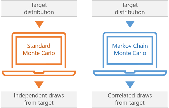
Markov Chain Monte Carlo (MCMC) methods are very powerful Monte Carlo methods that are often used in Bayesian inference.
While "classical" Monte Carlo methods rely on computer-generated samples made up of independent observations, MCMC methods are used to generate sequences of dependent observations. These sequences are Markov chains, which explains the name of the methods.
![]()
Table of contents
To understand MCMC, we need to be familiar with the basics of the Monte Carlo method.
We use the Monte Carlo method to approximate a feature of the probability
distribution of a random variable
![]() (e.g., its expected value), when we are not able to work it out analytically.
(e.g., its expected value), when we are not able to work it out analytically.
With a computer, we generate a sample
![]() of independent draws from the distribution of
of independent draws from the distribution of
![]() .
.
Then, we use the
empirical
distribution of the sample to carry out our calculations. The empirical
distribution is the discrete probability distribution that assigns probability
![]() to each one of the values
to each one of the values
![]() .
.
Example
If we need to compute the expected value of
![]() ,
we approximate it with the expected value of the empirical distribution, which
is just the sample mean of
,
we approximate it with the expected value of the empirical distribution, which
is just the sample mean of
![]() .
.
Example
If we need to calculate the probability that
![]() will be below some threshold, we approximate it with the fraction of
observations in the computer-generated sample that are below the threshold.
will be below some threshold, we approximate it with the fraction of
observations in the computer-generated sample that are below the threshold.
Example
To approximate the variance of
![]() ,
we compute the sample variance of
,
we compute the sample variance of
![]() .
.
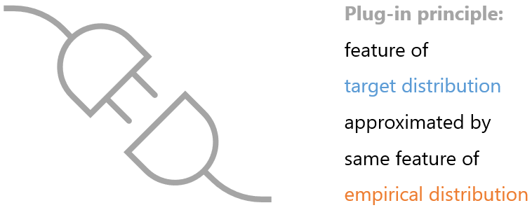
In general, whatever calculation we would like to perform on the true
distribution of
![]() is approximated by the corresponding calculation performed on the
empirical distribution. The latter is easy to perform on a
computer because it involves a discrete distribution with finite
support.
is approximated by the corresponding calculation performed on the
empirical distribution. The latter is easy to perform on a
computer because it involves a discrete distribution with finite
support.
This kind of procedure usually works well, in the sense that the approximation
converges to the true quantity as the sample size
![]() increases. This is known as the
plug-in principle.
increases. This is known as the
plug-in principle.
MCMC methods work like standard Monte Carlo methods, although with a twist:
the computer-generated draws
![]() are not independent, but they are serially correlated.
are not independent, but they are serially correlated.
In particular, they are the
realizations of
![]() random variables
random variables
![]() ,
...,
,
...,
![]() that form a Markov Chain.
that form a Markov Chain.
You do not need to be an expert about Markov Chains to use MCMC methods. A basic understanding of the material in the following sections suffices, although we recommend reading our introductory lecture on Markov chains.
A random sequence
![]() is a Markov chain if and only if, given the current value
is a Markov chain if and only if, given the current value
![]() ,
the future observations
,
the future observations
![]() are conditionally independent of the past values
are conditionally independent of the past values
![]() ,
for any positive integers
,
for any positive integers
![]() and
and
![]() .
.
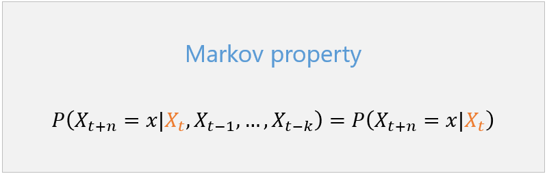
This property, known as the Markov property, says that the process is
memoryless: the probability distribution of the future values of the chain
depends only on its current value
![]() ,
regardless of how the value was reached (i.e., regardless of the path followed
by the chain in the past).
,
regardless of how the value was reached (i.e., regardless of the path followed
by the chain in the past).
Thanks to the Markov property, we basically need only two things to analyze a chain:
the conditional probabilities (or densities) that
![]() ,
given that
,
given that
![]() ,
denoted
by
,
denoted
by![]()
the unconditional probabilities that
![]() ,
denoted by
,
denoted by
![]()
Although this is not true in general of any Markov chain, the chains generated by MCMC methods have the following property:
two variables
![]() and
and
![]() are not
independent,
but they become closer and closer to being independent as
are not
independent,
but they become closer and closer to being independent as
![]() increases.
increases.
This property implies that
![]() converges to
converges to
![]() as
as
![]() becomes large.
becomes large.
This is very important. We usually generate the first value of the chain
(![]() )
in a somewhat arbitrary manner, but we know that the distribution of the terms
of the chain is less and less affected by our initial choice as
)
in a somewhat arbitrary manner, but we know that the distribution of the terms
of the chain is less and less affected by our initial choice as
![]() becomes large. In other words,
becomes large. In other words,
![]() converges to the same distribution
converges to the same distribution
![]() irrespective of how we choose
irrespective of how we choose
![]() .
.
In a chain generated by MCMC methods, not only
![]() converges to
converges to
![]() ,
but, as
,
but, as
![]() varies, the distributions
varies, the distributions
![]() become almost identical to each other. They converge to the so-called
stationary distribution of the chain.
become almost identical to each other. They converge to the so-called
stationary distribution of the chain.
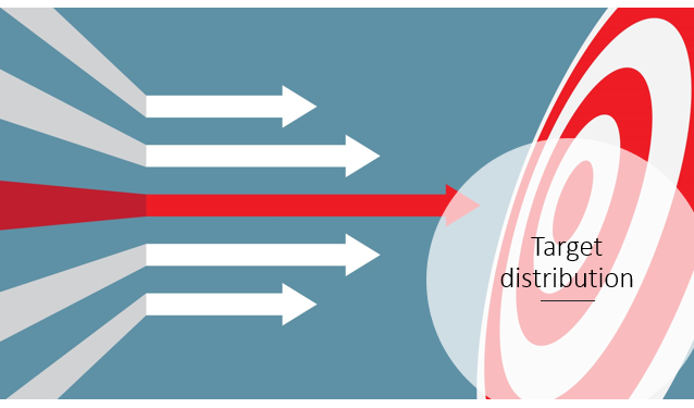
Moreover, the stationary distribution coincides with the target distribution, that is, the distribution from which we would like to extract a sample.
In other words, the larger
![]() is, the more
is, the more
![]() and
and
![]() are similar to the target distribution.
are similar to the target distribution.
Let us summarize what we have said thus far.
We can imagine an MCMC algorithm as a black box that takes two inputs:
an initial value
![]() ;
;
a target distribution.
The output is a sequence of values
![]() .
.
Although the first values of the sequence are extracted from distributions
that can be quite different from the target distribution, the similarity
between these distributions and the target progressively increases: when
![]() is large,
is large,
![]() is drawn from a distribution that is very similar to the target.
is drawn from a distribution that is very similar to the target.
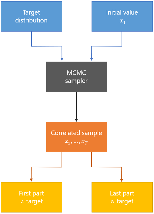
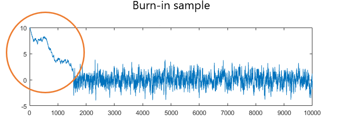
Because of the discrepancy between the target distribution and the distributions of the first terms of the chain, a common practice is to discard the first draws of an MCMC sample.
For example, if we have 110,000 draws, we discard the first 10,000 and keep the remaining 100,000.
The set of draws that are discarded is called the burn-in sample.
By discarding the burn-in sample, we eliminate draws whose distributions are far from the target distribution and we keep draws whose distributions are closer to the target.
This reduces the bias of any Monte Carlo approximation performed with the MCMC sample.
How to choose the size of the burn-in sample is discussed in the lecture on MCMC diagnostics.
After discarding a burn-in sample, we have a sample of draws from distributions that are very similar to the target.
However, we still have a problem: our draws are not independent.
What are the implications of the lack of independence?
To understand them, we need to go back to the standard Monte Carlo method.
The accuracy of a standard Monte Carlo simulation depends on the sample size
![]() :
the larger
:
the larger
![]() is, the better the approximation.
is, the better the approximation.
In the case of an MCMC simulation, we need to use the concept of
effective sample size:
![]() dependent observations are equivalent to a smaller number of independent
observations.
dependent observations are equivalent to a smaller number of independent
observations.
For example, 1000 dependent observations could be equivalent to 100 independent observations. In this case, we say that the effective sample size is equal to 100.
Roughly speaking, the higher the correlation between adjacent observations, the smaller the effective sample size, and the less accurate the MCMC approximation is.
This is why in an MCMC simulation, most of the efforts are devoted to reducing the correlation as much as possible, so as to achieve a satisfactory effective sample size.
Our lecture on MCMC diagnostics discusses this point in detail.
One of the most popular MCMC algorithms is the Metropolis-Hastings (M-H) algorithm.
Denote by
![]() the density (or mass) function of the target distribution,
that is, the distribution from which we wish to extract a sequence of draws.
the density (or mass) function of the target distribution,
that is, the distribution from which we wish to extract a sequence of draws.
For example,
![]() could be the posterior density in Bayesian inference.
could be the posterior density in Bayesian inference.
Denote by
![]() a conditional distribution from which we are able to extract
computer-generated samples (e.g., a multivariate normal distribution with mean
a conditional distribution from which we are able to extract
computer-generated samples (e.g., a multivariate normal distribution with mean
![]() ).
).
The generated sample
![]() ,
the value
,
the value
![]() on which we condition, and the argument of the target distribution
on which we condition, and the argument of the target distribution
![]() all have the same dimension.
all have the same dimension.
The M-H algorithm starts from any value
![]() belonging to the support
of the target distribution and generates the subsequent values
belonging to the support
of the target distribution and generates the subsequent values
![]() as follows:
as follows:
generate a proposal
![]() from the distribution
from the distribution
![]() ;
;
compute the acceptance
probability![[eq21]](/images/Markov-Chain-Monte-Carlo__65.png)
draw a uniform
random variable
![]() (on
(on
![]() );
);
if
![]() ,
accept the proposal and set
,
accept the proposal and set
![]() ;
otherwise, reject the proposal and set
;
otherwise, reject the proposal and set
![]() .
.
If some technical conditions are met, it can be proved that the distributions
of the draws
![]() converge to the target distribution
converge to the target distribution
![]() .
.
Furthermore,
![[eq23]](data:image/gif;base64,R0lGODlhAQABAIAAANvf7wAAACH5BAEAAAAALAAAAAABAAEAAAICRAEAOw==) where
where
![]() is
any function such that the expected value
is
any function such that the expected value
![]() exists and is finite, and
exists and is finite, and
![]() denotes almost sure
convergence as
denotes almost sure
convergence as
![]() tends to infinity.
tends to infinity.
In other words, a Strong Law of Large Numbers (an
ergodic theorem) holds
for the sample mean
![]() .
.
The power of the Metropolis-Hastings algorithm lies in the fact that you need
to know the function
![]() only up to a multiplicative constant.
only up to a multiplicative constant.
For example, in Bayesian inference it is very common to know the posterior distribution up to a multiplicative constant because the likelihood and the prior are known but the marginal distribution is not.
Suppose
that![]() and
we know
and
we know
![]() but not
but not
![]() .
.
Then, the acceptance probability in the M-H algorithm
is![[eq28]](/images/Markov-Chain-Monte-Carlo__83.png)
As a consequence, the acceptance probability, which is the only quantity that
depends on
![]() ,
can be computed without knowing the constant
,
can be computed without knowing the constant
![]() .
.
This is the beauty of the Metropolis-Hastings algorithm: we can generate draws from a distribution even if we do not fully know the density of that distribution!
For more details, see the lecture on the Metropolis-Hastings algorithm.
Another popular MCMC algorithm is the so-called Gibbs sampling algorithm.
Suppose that we want to generate draws of a random vector
![]() having joint
density
having joint
density![]() where
where
![]() are
are
![]() blocks of entries (or single entries) of
blocks of entries (or single entries) of
![]() .
.
Given a block
![]() ,
denote by
,
denote by
![]() the vector comprising all blocks except
the vector comprising all blocks except
![]() .
.
Suppose that we are able to generate draws from the
![]() conditional distributions
conditional distributions
![]() ,
...,
,
...,
![]() .
In MCMC jargon, these are called the full conditional
distributions.
.
In MCMC jargon, these are called the full conditional
distributions.
The Gibbs sampling algorithm starts from any vector
![]() belonging
to the support of the target distribution and generates the subsequent values
belonging
to the support of the target distribution and generates the subsequent values
![]() as follows:
as follows:
for
![]() ,
generate
,
generate
![]() from the conditional distribution with
density
from the conditional distribution with
density![]()
In other words, at each iteration, the blocks are extracted one by one from their full conditional distributions, conditioning on the latest draws of all the other blocks.
Note that at iteration
![]() ,
when you extract the
,
when you extract the
![]() -th
block, the latest draws of blocks
-th
block, the latest draws of blocks
![]() to
to
![]() are those already extracted in iteration
are those already extracted in iteration
![]() ,
while the latest draws of blocks
,
while the latest draws of blocks
![]() to
to
![]() are those extracted in the previous iteration
(
are those extracted in the previous iteration
(![]() ).
).
It can be proved that Gibbs sampling is a special case of Metropolis-Hastings.
Therefore, as in M-H, the distributions of the draws
![]() converge to the target distribution
converge to the target distribution
![]() .
Furthermore, an ergodic theorem for the sample means
.
Furthermore, an ergodic theorem for the sample means
![]() holds.
holds.
If you liked this lecture and you want to learn more about Markov Chain Monte Carlo methods, then we suggest that you read these two lectures:
Please cite as:
Taboga, Marco (2021). "Markov Chain Monte Carlo (MCMC) methods", Lectures on probability theory and mathematical statistics. Kindle Direct Publishing. Online appendix. https://www.statlect.com/fundamentals-of-statistics/Markov-Chain-Monte-Carlo.
Most of the learning materials found on this website are now available in a traditional textbook format.