Decision tree

We are now going to introduce decision trees, popular machine learning models that are also widely used as base learners in gradient boosting.

Table of contents

How decision trees work
Example
Terminology
Algorithms
Hyper-parameters
Use in gradient boosting
Missing values
Decision trees are linear regressions with dummies
Why decision trees
Statistical properties
Example: HICP dataset
References

How decision trees work

Decision trees are very simple predictive models:

we use the input variables (aka features) to classify the data into sub-groups satisfying certain binary conditions (e.g., all observations for which the first input $x_{1,t}$ is less than zero are in sub-group 1, and all the other observations are in sub-group 2);
we use the training sample to compute the sample mean of the output $y_{t}$ on each sub-group, which we then use as a constant prediction for all future observations that will be classified into that sub-group (e.g., if the sample mean of $y_{t}$ for all the observations belonging to the training sample and classified in sub-group 1 is 2.55, then any future observation classified in sub-group 1 will be predicted to have output equal to 2.55).

Remarks:

in a binary classification model, the sample mean of the output on a sub-group is a probability; in a multinoulli classification model, the sample mean of the output on a sub-group is a vector of probabilities;
the term decision tree is often reserved for trees used as classification models and used as a synonym of classification tree, while the term regression tree is used for trees used as regression models;
for concreteness, we have said above that the sample mean of $y_{y}$ on a sub-group is used as a prediction for future observations classified into that sub-group. This is not completely general: there are tree-construction algorithms where other statistics (e.g., the sample median) are used in place of the sample mean.

Example

In this example, two features are used to classify the data into three sub-groups.

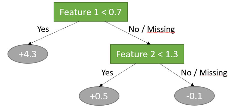
The three sub-groups are as follows:

all observations for which the first input is less than 0.7; the predicted output for this sub-group is 4.3;
all observations for which the first input is not less than 0.7 and the second input is less than 1.3; the predicted output for this sub-group is 0.5;
all observations for which the first input is not less than 0.7 and the second input is not less than 1.3; the predicted output for this sub-group is -0.1.

Note that also the observations whose inputs are missing are assigned to the sub-groups.

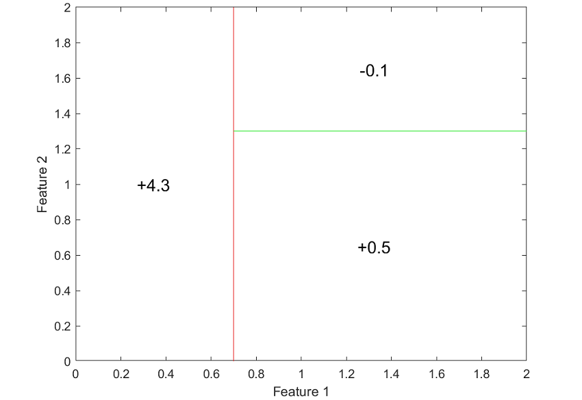
The next figure clearly shows how the decision tree subdivides the space of inputs into regions over which output predictions are constant.

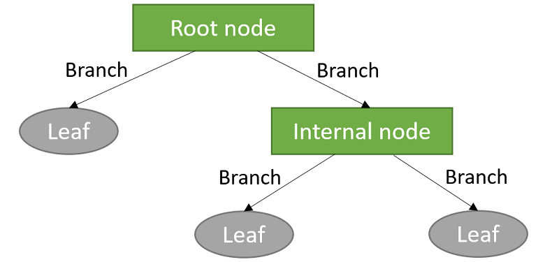
Example of a decision tree partitioning the input space

Terminology

The sub-groups are often called leaves, while intermediate splits that do not immediately lead to the formation of a leave are called internal nodes. The lines joining the various nodes and leaves are called branches.

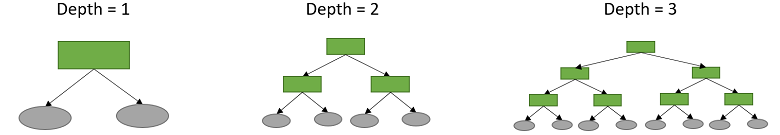
The structure of a decision tree: root node, internal nodes, branches, leaves

The largest number of splits made before reaching a leaf is called the depth of the tree.

Examples of depth-1, depth-2 and depth-3 trees

Algorithms

How do we choose the structure of the tree? How many branches? How many internal nodes and leaves? How do we select the inputs to use for the splits? How do we select the threshold value for each split (e.g., Feature 1 < 0.7 in the example above)?

These questions have no unique answer and many different algorithms for growing decision and regression trees have been proposed in the literature (see the Wikipedia article on decision tree learning for a review).

One of the most popular algorithms is CART (Classification And Regression Trees), which is used by the tree-training functions implemented in the scikit-learn package we are using. CART is a greedy algorithm that recursively splits sub-groups. The input variables and the thresholds used for the splits are chosen so as to minimize a measure of diversity among the output values included in a sub-group (e.g., variance for regression; entropy for classification).

In general, I would recommend not to re-invent the wheel and use the tree-construction algorithms implemented in standard machine-learning software, as they are usually highly optimized and thoroughly tested.

Hyper-parameters

Tree-construction algorithms usually have some hyper-parameters that allow us to control overfitting.

Two important hyper-parameters are:

maximum depth of the tree (the deeper the tree, the more likely it is to overfit);
minimum number of observations in a leaf (the lower the number of observations in a leaf, the more likely it is to overfit).

Use in gradient boosting

We often use decision trees as base learners in gradient boosting. Remember that base learners are usually required to be very simple models, affected as little as possible by overfitting. Therefore, what we usually do in gradient boosting is to train depth-2 decision trees (two internal nodes, four leaves), which are pretty simple but allow for interactions between input variables.

Missing values

An important detail about decision trees is how missing values are treated.

When an observation has a missing value for a certain input, and that input is used to classify the observation into one of two sub-groups, then the observation is assigned to the majority class (i.e., the sub-group that contains the largest number of observations from the training sample).

Although this imputation method obviously creates biases, it allows us to efficiently and automatically deal with missing values. Furthermore, when a decision tree is used as a base learner in a boosting algorithm, the biases created by this imputation method can be corrected by the other base learners (a sort of self-correction mechanism).

Decision trees are linear regressions with dummies

A decision tree can be seen as a linear regression of the output on some indicator variables (aka dummies) and their products.

In fact, each decision (input variable above/below a given threshold) can be represented by an indicator variable (1 if below, 0 if above).

In the example above, the tree

if $x_{1,t}<0.7$ , then ; else:
- if $x_{2,t}<1.3$ , then ; else

can be represented as [eq4] which in turn can be written as a constant plus a linear combination of the variables , , : [eq8]

Why decision trees

What is the main advantage of using decision trees to build predictive models?

When should we use decision trees instead of linear regressions?

The short answer is that decision trees, especially when used as base learners in a boosting algorithm, allow us to capture nonlinearities in the data that cannot be captured by linear regressions, for example:

non-linear effects (e.g., quadratic, cubic) of the inputs on the output;
non-linear interactions among inputs (e.g., products, ratios);
threshold effects (an input has an effect on the output only if it is above a given level);
regime switches (e.g., if the value of an input variable exceeds a threshold, then the effect of another variable changes).

Moreover, decision trees can automatically deal with missing values.

Statistical properties

Note that, by building a decision tree, we partition the input space into regions over which is constant; in each region, the constant is equal to the average output over that region.

Thus, is similar to the Nadaraya-Watson kernel regression estimator of the conditional expected value of $y_{t}$ given $x_{t}$ . The only difference is that the kernel density estimator is replaced by the naive density estimator described by Fix and Hodges (1951) and Pagan and Ullah (1999). By using arguments similar to those used for the Nadaraya-Watson estimator, it is possible to prove that converges to the expected value of $y_{t}$ given $x_{t}$ (which is the best possible prediction of $y_{t}$ given $x_{t}$ ) as the sample size goes to infinity and the complexity of the tree increases.

This probably sounds too technical, but the bottom line is: decision/regression trees not only work well in practice, but they are theoretically sound, as they enjoy good asymptotic properties. Their predictions converge to the best possible predictions!

Example: HICP dataset

We are going to train a regression tree on the same inflation dataset used previously.

We will use the squared error as a loss function.

Import the data and use scikit-learn to split into train-test1-test2 (60-20-20)

We are going to train a single model and we will do no model selection. Therefore, we will not need a validation set. We instead create two test sets. Shortly you will understand why.

# Import the packages used to load and manipulate the data
import numpy as np # Numpy is a Matlab-like package for array manipulation and linear algebra
import pandas as pd # Pandas is a data-analysis and table-manipulation tool
import urllib.request # Urlib will be used to download the dataset

# Import the function that performs sample splits from scikit-learn
from sklearn.model_selection import train_test_split

# Load the output variable with pandas (download with urllib if not downloaded previously)
remoteAddress = 'https://www.statlect.com/ml-assets/y_hicp.csv'
localAddress = './y_hicp.csv'
try:
    y = pd.read_csv(localAddress, header=None)
except:
    urllib.request.urlretrieve(remoteAddress, localAddress)
    y = pd.read_csv(localAddress, header=None)
y = y.values # Transform y into a numpy array

# Print some information about the output variable
print('Class and dimension of output variable:')
print(type(y))
print(y.shape)

# Load the input variables with pandas 
remoteAddress = 'https://www.statlect.com/ml-assets/x_hicp.csv'
localAddress = './x_hicp.csv'
try:
    x = pd.read_csv(localAddress, header=None)
except:
    urllib.request.urlretrieve(remoteAddress, localAddress)
    x = pd.read_csv(localAddress, header=None)
x = x.values

# Print some information about the input variables
print('Class and dimension of input variables:')
print(type(x))
print(x.shape)

# Create the training sample
x_train, x_test_1_test_2, y_train, y_test_1_test_2 
  = train_test_split(x, y, test_size=0.4, random_state=1)

# Split the remaining observations into two test samples
x_test_1, x_test_2, y_test_1, y_test_2 
  = train_test_split(x_test_1_test_2, y_test_1_test_2, test_size=0.5, random_state=1) 

# Print the numerosities of the three samples
print('Numerosities of training, validation and test samples:')
print(x_train.shape[0], x_test_1.shape[0], x_test_2.shape[0])

The output is:

Class and dimension of output variable:
class 'numpy.ndarray'
(270, 1)
Class and dimension of input variables:
class 'numpy.ndarray'
(270, 113)
Numerosities of training, validation and test samples:
162 54 54

Train a single tree

We now train a regression tree with all the 113 input variables.

We set the maximum depth of the tree to 4.

# Import functions for tree fitting and model evaluation
from sklearn.tree import DecisionTreeRegressor
from sklearn.metrics import mean_squared_error, r2_score

# Create a regression tree object
tree = DecisionTreeRegressor(criterion='mse', max_depth=4, random_state=10)

# Train the model 
tree.fit(x_train, y_train)

# Make predictions on the train and test sets
y_train_pred = tree.predict(x_train)[..., np.newaxis]
y_test_1_pred = tree.predict(x_test_1)[..., np.newaxis]
y_test_2_pred = tree.predict(x_test_2)[..., np.newaxis]

# Print empirical risk on the train and test sets
print('MSE on training set:')
print(mean_squared_error(y_train, y_train_pred))
print('MSE on test set 1:')
print(mean_squared_error(y_test_1, y_test_1_pred))
print('MSE on test set 2:')
print(mean_squared_error(y_test_2, y_test_2_pred))
print('')

# Print R squared on all sets
print('R squared on training set:')
print(r2_score(y_train, y_train_pred))
print('R squared on test set 1:')
print(r2_score(y_test_1, y_test_1_pred))
print('R squared on test set 2:')
print(r2_score(y_test_2, y_test_2_pred))

The output is:

MSE on training set:
0.02851595628573428
MSE on test set 1:
0.06748511269138653
MSE on test set 2:
0.10848735618948044

R squared on training set:
0.8186516532644803
R squared on test set 1:
0.7145085505718741
R squared on test set 2:
0.4768175397186226

Discussion of results

By chance, we got something that often happens with a single decision tree.

We obtained an impressive performance on test_set_1 (better than any model we have trained thus far), but the performance was much lower on test_set_2. Obtaining very different performances on different test sets is something that often happens with decision trees, as they are known to be non-robust, especially if there are leaves containing few observations.

In the next section we re-run the code by requiring that each leaf should contain at least 10 observations.

Train the same tree with min_samples_leaf = 10

# Create a regression tree object
tree = DecisionTreeRegressor(criterion='mse', random_state=10, max_depth=4, min_samples_leaf=10)

# Train the model 
tree.fit(x_train, y_train)

# Make predictions on the train and test sets
y_train_pred = tree.predict(x_train)[..., np.newaxis]
y_test_1_pred = tree.predict(x_test_1)[..., np.newaxis]
y_test_2_pred = tree.predict(x_test_2)[..., np.newaxis]

# Print empirical risk on the train and test sets
print('MSE on training set:')
print(mean_squared_error(y_train, y_train_pred))
print('MSE on test set 1:')
print(mean_squared_error(y_test_1, y_test_1_pred))
print('MSE on test set 2:')
print(mean_squared_error(y_test_2, y_test_2_pred))
print('')

# Print R squared on all sets
print('R squared on training set:')
print(r2_score(y_train, y_train_pred))
print('R squared on test set 1:')
print(r2_score(y_test_1, y_test_1_pred))
print('R squared on test set 2:')
print(r2_score(y_test_2, y_test_2_pred))

The output is:

MSE on training set:
0.04985658826665274
MSE on test set 1:
0.07912753888113853
MSE on test set 2:
0.09212393895189586

R squared on training set:
0.6829350639538556
R squared on test set 1:
0.6652560118234798
R squared on test set 2:
0.5557304489245373

The performance is more homogeneous across the two test sets.

Plot the tree

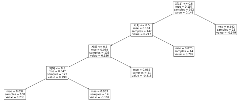
Let us see what the tree looks like.

# Import packages and functions needed to plot a tree
from sklearn.tree import plot_tree
from matplotlib import pyplot as plt

# Plot the tree
plt.figure(figsize=(24,9), dpi=600)
fig=plot_tree(tree, fontsize=12)
plt.show()

The output is:

References

Fix, E. and Hodges Jr, J.L., 1951. Discriminatory analysis-nonparametric discrimination: consistency properties. California Univ., Berkeley.

Pagan, A. and Ullah, A., 1999. Nonparametric econometrics. Cambridge university press.

How to cite

Please cite as:

Taboga, Marco (2021). "Decision tree", Lectures on machine learning. https://www.statlect.com/machine-learning/decision-tree.