Overfitting

Machine learning methods are very good at dealing with overfitting, that is, the tendency of statistical models to accurately fit previously seen data and to poorly predict previously unseen data.

Table of contents

Parametric models
Mathematics of overfitting
Overfitting and model complexity
Curse of dimensionality
Bias-variance decomposition
Overfitting in linear regressions estimated by OLS
Sample size

Parametric models

Remember that we have defined a predictive model as a function that takes an input $x_{t}$ as argument and returns a prediction $widetilde{y}_{t}$ of the true output $y_{t}$ .

In what follows, we are going to deal with parametric models, that is, families of models indexed by a parameter vector .

In a parametric model, predicted outputs depend on the parameter and so do losses , the risk and the empirical risk .

Typical examples of parametric models are:

a linear regression model where the input $x_{t}$ is a row vector and the parameter is a vector of regression coefficients;
a logistic classification model where is the logistic function.

Mathematics of overfitting

When we estimate the parameter naively by empirical risk minimization, we search for a solution of the problem

But this is equivalent to

Thus, we are minimizing the sum of two terms:

the true risk of the predictive model ;
the term , which is a measure of the reliability of the empirical risk as an estimate of the true risk . The smaller this term is, the more under-estimates the true risk (the less its reliability).

Clearly, we would like to minimize only the first term, while minimizing the second one (reliability) is detrimental. Unfortunately, we are minimizing both!

There is no general way to tell how much the second term contributes to the minimum we attain, but in certain cases its contribution can be substantial. In other words, our estimate of the expected loss, performed with the same sample used to estimate , can be over-optimistic. This is called overfitting.

In the above formulae, we can replace with , the average loss on a sample (so-called test sample) different from the one used to estimate (so-called estimation or training sample). By doing so, we can see that, when we perform empirical risk minimization naively, we are also maximizing the disappointment experienced on the test sample.

Another way to see the overfitting problem is that the empirical risk provides a biased estimate of the true risk when it is computed with the same sample used to train our models.

Important: when the predictive model is a linear regression model and the loss function is the squared error, then naive empirical risk minimization is the same as OLS (ordinary least squares) estimation. In this case the bias of the empirical risk can be derived analytically.

What machine learning does: in the typical machine learning workflow, overfitting is constantly kept under control during the minimization process, so as to avoid it as much as possible.

Overfitting and model complexity

Typically, but not necessarily, overfitting tends to be more severe when models are highly complex (i.e., the dimension of the parameter vector is large).

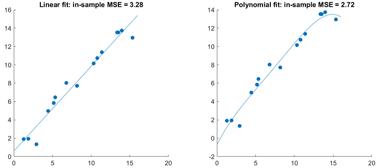
A classical example is provided by a simple linear regression of few data points on time vs a more complex linear regression on time and several of its powers (polynomial terms).

A more complex model typically has better in-sample performance...

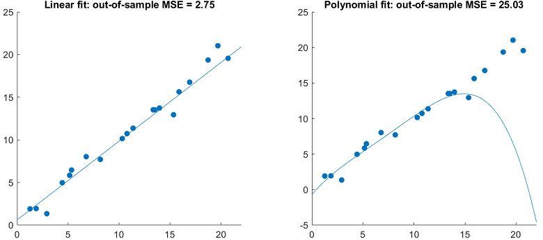
... but worse out-sample performance

... leads to inaccurate out-of-sample predictions.

Curse of dimensionality

A reason why models with many parameters tend to overfit is that they are affected by the so-called curse of dimensionality.

For concreteness, suppose that the number of parameters is the same as the number of output variables, as in linear regression (where the number of regressors is equal to the number of regression coefficients, which are the parameters to be estimated).

The percentage of regions of the space of outputs covered by our data set decreases exponentially in the number of outputs (and parameters).

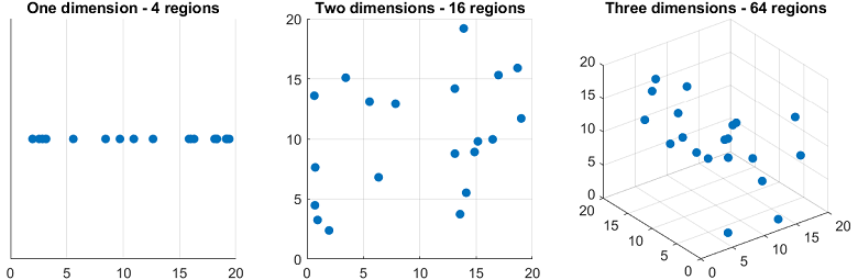
Coverage of the space decreases exponentially in the number of dimensions.

As a consequence, as we increase the dimensionality of our model, we increase the probability that new data points (out-of-sample data) will belong to regions of space that were not covered by the training/estimation data and where things may work very differently than in the regions that were covered.

This exponential decrease in coverage is called curse of dimensionality.

A related phenomenon is that the average distance between new points and the points belonging to the estimation sample tends to increase with the dimension of the model.

Bias-variance decomposition

Further insights about the possible pitfalls of highly parametrized models can be derived from the so-called bias-variance decomposition.

Suppose that the loss function is the squared error.

Then, the best possible prediction of $y_{t}$ is the conditional expectation

It can be proved that [eq18] which is called bias-variance decomposition.

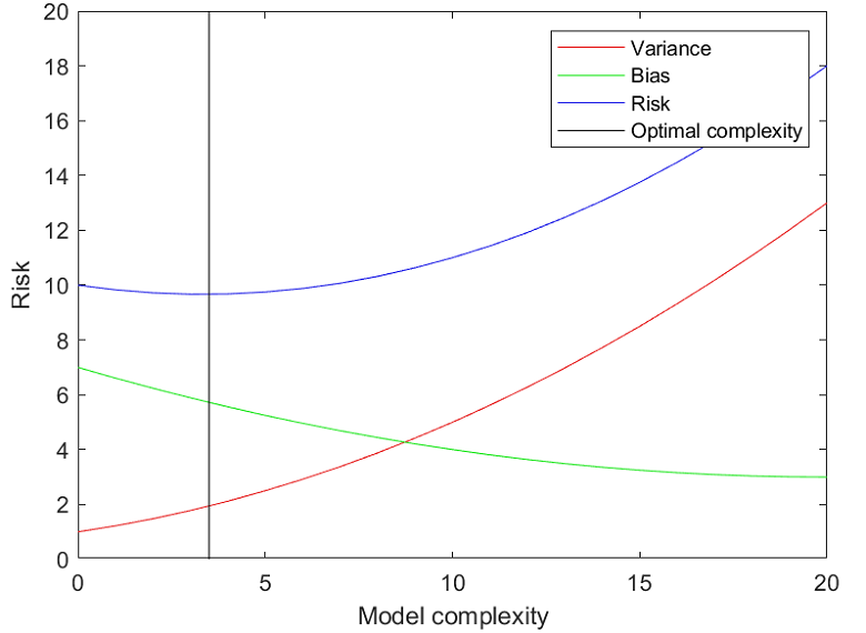
In other words, the risk of a model is the sum of three terms:

the irreducible error, due to the fact that $x_{t}$ may not contain all the information that is needed to perfectly predict $y_{t}$ ;
the bias, generated by systematic differences between the model predictions $widetilde{y}_{t}$ and the best possible predictions $y_{t}^{st }$ ;
the variance, due to the fact that the parameters of our predictive models and hence the predictions $widetilde{y}_{t}$ are affected by sampling variability.

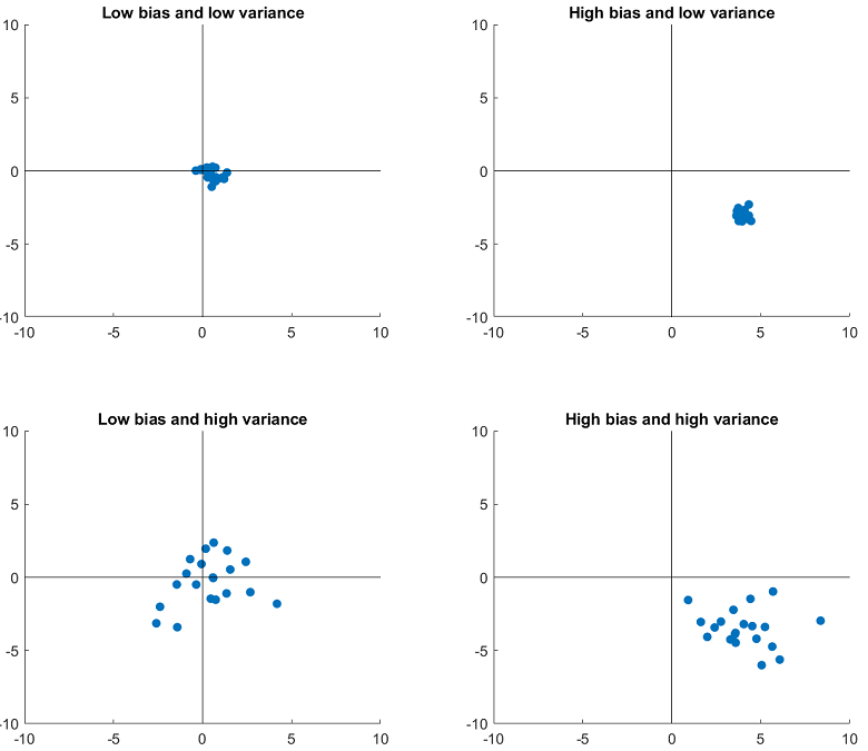
It turns out that in many settings variance is an increasing function of model complexity (number of parameters), while bias is a decreasing function. As a consequence, there is a trade-off between the two.

Beyond the point of optimal balance between the two (i.e., if complexity is increased too much), performance degrades.

Illustration of the trade-off between bias and variance.

Overfitting in linear regressions estimated by OLS

In linear regression with regressors (and zero-mean variables), the true vector of regression coefficients is where:

$Sigma _{xx}$ is the covariance matrix of inputs $x_{t}$ ;
$sigma _{xy}$ is the vector of covariances between inputs $x_{t}$ and outputs $y_{t}$ .

The OLS estimator is where the matrix and the vector are obtained by stacking inputs and outputs.

Roughly speaking, $X^{ op}X$ estimates $Sigma_{xx}$ and $X^{ op}y$ estimates $sigma_{xy}$ .

The number of covariances to estimate (and potential sources of error in estimating ) is . Hence, it grows with $K^{2}$ .

The fact that the sources of error grow with the square of the number of parameters is one of the reasons why OLS regressions with many regressors overfit data and work poorly (unless you have tons of data).

Sample size

An important thing to note is that all of the aforementioned problems are very severe with small sample sizes, but they tend to become less severe when the sample size increases:

empirical risk tends to become a more reliable estimate of true risk (by the Law of Large Numbers); hence, over-fitting decreases;
the curse of dimensionality becomes less of a problem (because more and more regions of space are covered by the sample);
the variance (in the bias-variance decomposition) decreases because there is less sampling variability.

How to cite

Please cite as:

Taboga, Marco (2021). "Overfitting", Lectures on machine learning. https://www.statlect.com/machine-learning/overfitting.