K-fold cross-validation

Until now we have used the simplest of all cross-validation methods, which consists in testing our predictive models on a subset of the data (the test set) that has not been used for training or selecting the predictive models. This simple cross-validation method is sometimes called the holdout method.

There are more sophisticated cross-validation methods that allow us to obtain better predictive models, together with accurate estimates of an upper bound on the expected loss. In these methods, we perform multiple different partitions of the data into training, validation and test sets, we build a different predictive model for each partition, and finally we average the predictions made by the various models (so-called ensembling).

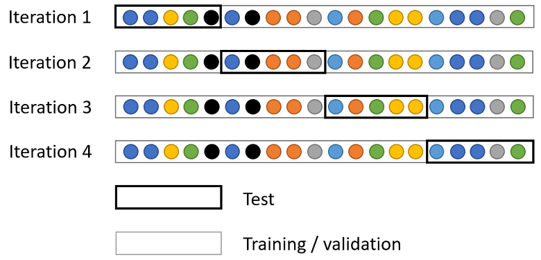
Here we introduce the most popular of these methods, called K-fold cross-validation.

Table of contents

Folds
Ensembling
Advantages and disadvantages
Python example

Folds

The data is divided into subsets, called folds. Each fold contains (approximately) the same number of observations.

Then, for $k=1,\ldots ,K$ , we use the -th fold (denoted by $au _{k}$ ) as the test set and use the remaining folds to train a predictive model .

Graphical representation of how the data is split in 4 folds over 4 iterations

For each fold, we compute the estimate of the expected loss [eq2] where $x_{t}$ is a vector of inputs, is the loss incurred by using as a forecast of the observed output $y_{t}$ , and is the number of observations in the -th fold.

Remark: the folds used to train a predictive model can be divided into training and validation sets if we need a validation set for model selection.

Ensembling

After training the models , we use their ensemble average as our final prediction [eq7]

We then compute the average loss [eq8]

As previously discussed, this average is an estimate of an upper bound on the expected loss of the ensemble average (remember that the expected loss of the ensemble average equals the average expected loss of the models in the ensemble minus a correction term that measures the diversity of the models in the ensemble).

Advantages and disadvantages

K-fold cross validation is straightforward to implement: once we have a routine for training a predictive model, we just run it times on the different partitions of the data. The only real disadvantage is the computational cost.

As a reward for facing an increased computational cost, we have two main advantages:

our final model (the ensemble average) has been trained on all the data (no data have been "wasted") and it enjoys some benefits from ensembling;
although we no longer have an unbiased estimate of the expected loss of the final model, is an estimate of an upper bound to it, which uses all the data in the sample and should therefore be pretty precise.

Python example

Let us use K-fold cross-validation to improve on the simpler holdout cross-validation performed when we built a single boosted tree to predict the output variable in an artificially-generated data set.

Import the data

# Import the packages used to load and manipulate the data
import numpy as np # Numpy is a Matlab-like package for array manipulation and linear algebra
import pandas as pd # Pandas is a data-analysis and table-manipulation tool
import urllib.request # Urlib will be used to download the dataset

# Import the function that performs sample splits from scikit-learn
from sklearn.model_selection import train_test_split

# Load the output variable with pandas (download with urllib if not downloaded previously)
remoteAddress = 'https://www.statlect.com/ml-assets/y_artificial.csv'
localAddress = './y_artificial.csv'
try:
    y = pd.read_csv(localAddress, header=None)
except:
    urllib.request.urlretrieve(remoteAddress, localAddress)
    y = pd.read_csv(localAddress, header=None)
y = y.values # Transform y into a numpy array

# Print some information about the output variable
print('Class and dimension of output variable:')
print(type(y))
print(y.shape)

# Load the input variables with pandas 
remoteAddress = 'https://www.statlect.com/ml-assets/x_artificial.csv'
localAddress = './x_artificial.csv'
try:
    x = pd.read_csv(localAddress, header=None)
except:
    urllib.request.urlretrieve(remoteAddress, localAddress)
    x = pd.read_csv(localAddress, header=None)
x = x.values

# Print some information about the input variables
print('Class and dimension of input variables:')
print(type(x))
print(x.shape)

The output is:

Class and dimension of output variable:
class 'numpy.ndarray'
(500, 1)
Class and dimension of input variables:
class 'numpy.ndarray'
(500, 300)

Run the K-fold cross-validation on LightGBM boosted trees

We create 5 folds using the KFold class provided by the scikit-learn package.

Then, we use LightGBM to make predictions on each fold.

#Import the lightGBM package
import lightgbm as lgb

# Import the functions that performs sample splits from scikit-learn
from sklearn.model_selection import train_test_split, KFold

# Import model-evaluation metrics from scikit-learn
from sklearn.metrics import mean_squared_error, r2_score

# Set number of folds and ensemble variables
n_folds = 5
ensemble = []
mses_single_models = []
mses_constant_predictions = []
r_squareds_single_models = []

# Initialize k_fold splitter
K_fold = KFold(n_splits=n_folds, random_state=0, shuffle=True)

# Iterate over folds
for train_val_index, test_index in K_fold.split(x):
    # Get train_val (K-1 folds) and test (1 fold)
    x_train_val, x_test = x[train_val_index], x[test_index]
    y_train_val, y_test = y[train_val_index], y[test_index] 
    
    # Partition the train_val set
    x_train, x_val, y_train, y_val 
      = train_test_split(x_train_val, y_train_val, test_size=0.25, random_state=0)
    
    # Prepare dataset in LightGMB format
    y_train = np.squeeze(y_train)
    y_val = np.squeeze(y_val)
    train_set = lgb.Dataset(x_train, y_train, silent=True)
    valid_set = lgb.Dataset(x_val, y_val, silent=True)
    
    # Set algorithm parameters
    params = {
        'objective': 'regression',
        'learning_rate': 0.10,
        'metric': 'mse',
        'nthread': 8,
        'min_data_in_leaf': 10,
        'max_depth': 2,
        'verbose': -1
    }
    
    # Train the model 
    boosted_tree = lgb.train(
        params = params,
        train_set = train_set,
        valid_sets = valid_set,
        num_boost_round = 10000,
        early_stopping_rounds =  20,
        verbose_eval = False,
    )
    
    # Save the model in the ensemble list
    ensemble.append(boosted_tree)
    
    # Make predictions on test and compute performance metrics
    y_test_pred = boosted_tree.predict(x_test)
    mses_single_models.append(mean_squared_error(y_test, y_test_pred))
    mses_constant_predictions.append(mean_squared_error(y_test, 0*y_test + np.mean(y_train)))
    r_squareds_single_models.append(r2_score(y_test, y_test_pred))

# Print performance metrics on test sample
print('Test MSEs of models in the ensemble:')
print(mses_single_models)
print('Test MSEs of constant predictions equal to sample mean on training set:')
print(mses_constant_predictions)
print('Average test MSE of models in the ensemble:')
print(np.mean(mses_single_models))
print('')

print('Test R squareds of models in the ensemble:')
print(r_squareds_single_models)
print('Average test R squared of models in the ensemble:')
print(np.mean(r_squareds_single_models))

The output is:

Test MSEs of models in the ensemble:
[74.57708434382333, 37.439965145009516, 16.801894170417487, 54.55429632149937, 30.007456926513534]
Test MSEs of constant predictions equal to sample mean on training set:
[293.2026939915153, 167.6726253022108, 104.80130552664033, 213.67954000052373, 131.20844137862687]
Average test MSE of models in the ensemble:
42.67613938145264

Test R squareds of models in the ensemble:
[0.7414010556669601, 0.7762513029977958, 0.8356878267813256, 0.7416211645498416, 0.7712684886703587]
Average test R squared of models in the ensemble:
0.7732459677332564

There is significant variation in test mean squared errors (MSEs) across the folds, although it is mostly due to differences in variance (test MSEs of constant predictions). The R squareds are more homogeneous, that is, the proportion of variance explained by the predictions is more stable across folds.

Anyway, the variability in test MSEs reveals that it was probably a good idea to run a K-fold cross-validation.

At this stage, it is not possible to say anything more precise about the benefits from using K-fold cross-validation instead of the simple holdout method (although there are good theoretical guarantees about them). The benefits are likely to become apparent when we put the model in production, which we simulate below.

Put the model in production

We now see how our predictive model performs in production, on new data that becomes available after we have completed the training.

# Load the input and output variables with pandas 
y_production = pd.read_csv('./assets/y_artificial_production.csv', header=None)
y_production = y_production.values
y_production = np.squeeze(y_production)
x_production = pd.read_csv('./assets/x_artificial_production.csv', header=None)
x_production = x_production.values

# Initialize ensemble variables on production dataset
y_production_pred_ensemble = 0
production_mses_single_models = []
production_r_squareds_single_models = []

# Make predictions with all models in the ensemble and compute ensemble average
for model in ensemble:
    y_production_pred = model.predict(x_production)
    production_mses_single_models.append(mean_squared_error(y_production, y_production_pred))
    production_r_squareds_single_models.append(r2_score(y_production, y_production_pred))
    y_production_pred_ensemble += y_production_pred/n_folds

# Print MSEs    
print('Production MSEs of models in the ensemble:')
print(production_mses_single_models)
print('Average production MSE of models in the ensemble:')
print(np.mean(production_mses_single_models))
print('Production MSE of ensemble average:')
print(mean_squared_error(y_production, y_production_pred_ensemble))
print('')

# Print R squareds
print('Production R squareds of models in the ensemble:')
print(production_r_squareds_single_models)
print('Average production R squared of models in the ensemble:')
print(np.mean(production_r_squareds_single_models))
print('Production R squared of ensemble average:')
print(r2_score(y_production, y_production_pred_ensemble))

The output is:

Production MSEs of models in the ensemble:
[39.64176656361246, 32.90628594145072, 37.6388748646386, 44.169307277678485, 43.86534683792454]
Average production MSE of models in the ensemble:
39.64431629706096
Production MSE of ensemble average:
33.64136466519085

Production R squareds of models in the ensemble:
[0.7639469310457051, 0.8040543987387033, 0.7758734614027009, 0.736986985185174, 0.73879696493291]
Average production R squared of models in the ensemble:
0.7639317482610387
Production R squared of ensemble average:
0.7996772580685613

This is an excellent result! The performance of the ensemble average is significantly better than the average performance of the models in the ensemble.

How to cite

Please cite as:

Taboga, Marco (2021). "K-fold cross-validation", Lectures on machine learning. https://www.statlect.com/machine-learning/k-fold-cross-validation.