Linear correlation is a measure of dependence between two random variables.
It has the following characteristics:
it ranges between -1 and 1;
it is proportional to covariance;
its interpretation is very similar to that of covariance (see here).
![]()
Let
![]() and
and
![]() be two random variables.
be two random variables.
The linear correlation coefficient (or Pearson's correlation
coefficient) between
![]() and
and
![]() is
is
![[eq1]](data:image/gif;base64,R0lGODlhAQABAIAAANvf7wAAACH5BAEAAAAALAAAAAABAAEAAAICRAEAOw==) where:
where:
![]() is the covariance between
is the covariance between
![]() and
and
![]() ;
;
![]() and
and
![]() are the standard deviations of
are the standard deviations of
![]() and
and
![]() .
.
The linear correlation coefficient is well-defined only as long as
![]() ,
,
![]() and
and
![]() exist and are well-defined.
exist and are well-defined.
It is often denoted by
![]() .
.
In principle, the ratio is well-defined only if
![]() and
and
![]() are strictly greater than zero.
are strictly greater than zero.
However, it is often assumed that
![]() when one of the two standard deviations is zero.
when one of the two standard deviations is zero.
This is equivalent to assuming that
![]() because
because
![]() when one of the two standard deviations is zero.
when one of the two standard deviations is zero.
The interpretation is similar to the interpretation of covariance: the
correlation between
![]() and
and
![]() provides a measure of how similar their deviations from the respective means
are (see the lecture on Covariance for a detailed
explanation).
provides a measure of how similar their deviations from the respective means
are (see the lecture on Covariance for a detailed
explanation).
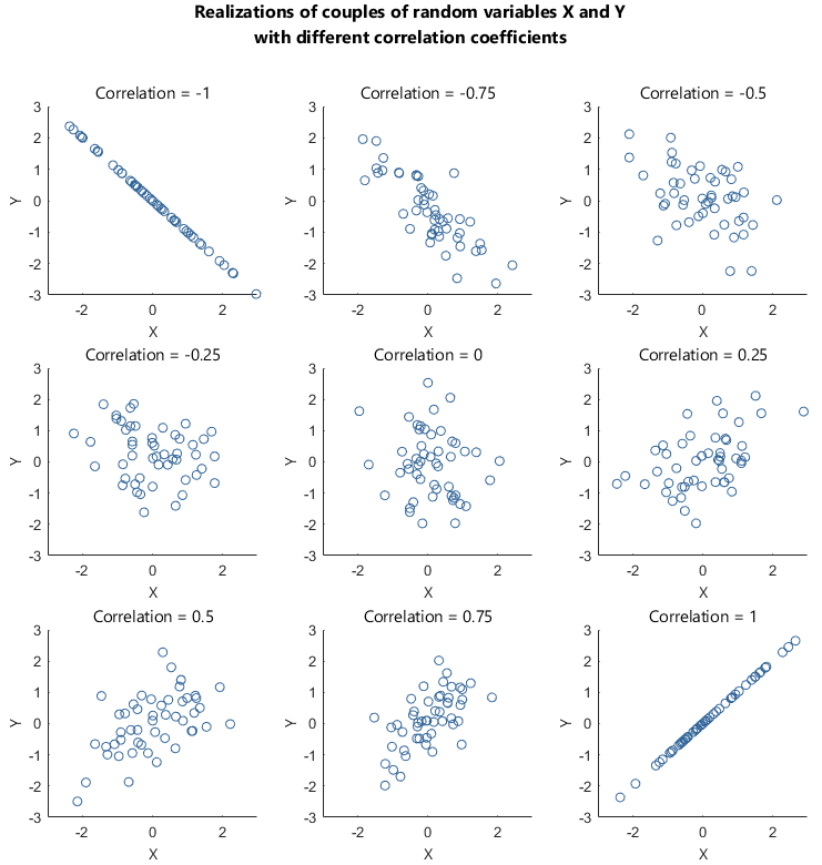
Linear correlation ranges between
![]() and
and
![]() :
:![]()
Thanks to this property, correlation allows us to easily understand the intensity of the linear dependence between two random variables:
the closer correlation is to
![]() ,
the stronger the positive linear dependence between
,
the stronger the positive linear dependence between
![]() and
and
![]() is;
is;
the closer it is to
![]() ,
the stronger the negative linear dependence between
,
the stronger the negative linear dependence between
![]() and
and
![]() is.
is.
The following terminology is often used:
If
![]() then
then
![]() and
and
![]() are said to be positively linearly correlated (or simply
positively correlated).
are said to be positively linearly correlated (or simply
positively correlated).
If
![]() then
then
![]() and
and
![]() are said to be negatively linearly correlated (or simply
negatively correlated).
are said to be negatively linearly correlated (or simply
negatively correlated).
If
![]() then
then
![]() and
and
![]() are said to be linearly correlated (or simply
correlated).
are said to be linearly correlated (or simply
correlated).
If
![]() then
then
![]() and
and
![]() are said to be uncorrelated. Also note that
are said to be uncorrelated. Also note that
![]()
![]() .
Therefore, two random variables
.
Therefore, two random variables
![]() and
and
![]() are uncorrelated whenever
are uncorrelated whenever
![]() .
.
In this example we show how to compute the coefficient of linear correlation between two discrete random variables.
Let
![]() be a
be a
![]() -dimensional
random vector and denote its entries by
-dimensional
random vector and denote its entries by
![]() and
and
![]() .
.
Let the support of
![]() be
be
![]() and
its joint probability
mass function
be
and
its joint probability
mass function
be
The support of
![]() is
is![]() and
its probability mass
function
is
and
its probability mass
function
is
The expected value of
![]() is
is
The expected value of
![]() is
is
The variance of
![]() is
is
The standard deviation of
![]() is
is
The support of
![]() is:
is:![]() and
its probability mass function
is
and
its probability mass function
is
The expected value of
![]() is
is
The expected value of
![]() is
is
The variance of
![]() is
is
The standard deviation of
![]() is
is
Using the transformation
theorem, we can compute the expected value of
![]() :
:![[eq34]](/images/linear-correlation__80.png)
Hence, the covariance between
![]() and
and
![]() is
is![]() and
the linear correlation coefficient
is
and
the linear correlation coefficient
is![[eq36]](/images/linear-correlation__84.png)
The following sections contain more details about the linear correlation coefficient.
Let
![]() be a random variable,
then
be a random variable,
then![]()
This is proved as
follows:where
we have used the fact
that![]()
The linear correlation coefficient is
symmetric:![]()
This is proved as
follows:where
we have used the fact that covariance is
symmetric:![]()
Below you can find some exercises with explained solutions.
Let
![]() be a
be a
![]() discrete random vector and denote its components by
discrete random vector and denote its components by
![]() and
and
![]() .
.
Let the support of
![]() beand
its joint probability mass function
be
beand
its joint probability mass function
be
Compute the coefficient of linear correlation between
![]() and
and
![]() .
.
The support of
![]() is
is![]() and
its marginal
probability mass function
isThe
expected value of
and
its marginal
probability mass function
isThe
expected value of
![]() isThe
expected value of
isThe
expected value of
![]() isThe
variance of
isThe
variance of
![]() isThe
standard deviation of
isThe
standard deviation of
![]() isThe
support of
isThe
support of
![]() is
is![]() and
its marginal probability mass function
isThe
expected value of
and
its marginal probability mass function
isThe
expected value of
![]() isThe
expected value of
isThe
expected value of
![]() isThe
variance of
isThe
variance of
![]() isThe
standard deviation of
isThe
standard deviation of
![]() isUsing
the transformation theorem, we can compute the expected value of
isUsing
the transformation theorem, we can compute the expected value of
![]() :Hence,
the covariance between
:Hence,
the covariance between
![]() and
and
![]() isand
the coefficient of linear correlation between
isand
the coefficient of linear correlation between
![]() and
and
![]() is
is
Let
![]() be a
be a
![]() discrete random vector and denote its entries by
discrete random vector and denote its entries by
![]() and
and
![]() .
.
Let the support of
![]() beand
its joint probability mass function
be
beand
its joint probability mass function
be
Compute the coefficient of linear correlation between
![]() and
and
![]() .
.
The support of
![]() is
is![]() and
its marginal probability mass function
isThe
mean of
and
its marginal probability mass function
isThe
mean of
![]() isThe
expected value of
isThe
expected value of
![]() isThe
variance of
isThe
variance of
![]() isThe
standard deviation of
isThe
standard deviation of
![]() isThe
support of
isThe
support of
![]() is
is![]() and
its probability mass function
isThe
mean of
and
its probability mass function
isThe
mean of
![]() isThe
expected value of
isThe
expected value of
![]() isThe
variance of
isThe
variance of
![]() isThe
standard deviation of
isThe
standard deviation of
![]() isThe
expected value of the product
isThe
expected value of the product
![]() can
be derived using the transformation
theorem
can
be derived using the transformation
theorem![[eq74]](/images/linear-correlation__163.png) Therefore,
putting pieces together, the covariance between
Therefore,
putting pieces together, the covariance between
![]() and
and
![]() isand
the coefficient of linear correlation between
isand
the coefficient of linear correlation between
![]() and
and
![]() is
is
Let
![]() be a continuous
random vector with support
be a continuous
random vector with support
![]() and
let its joint probability density function
be
and
let its joint probability density function
be![[eq79]](/images/linear-correlation__172.png)
Compute the coefficient of linear correlation between
![]() and
and
![]() .
.
The support of
![]() is
is![]() When
When
![]() ,
the marginal
probability density function of
,
the marginal
probability density function of
![]() is
is
![]() ,
while, when
,
while, when
![]() ,
the marginal probability density function of
,
the marginal probability density function of
![]() can be obtained by integrating
can be obtained by integrating
![]() out of the joint probability density as
follows:Thus,
the marginal probability density function of
out of the joint probability density as
follows:Thus,
the marginal probability density function of
![]() isThe
expected value of
isThe
expected value of
![]() isThe
expected value of
isThe
expected value of
![]() isThe
variance of
isThe
variance of
![]() isThe
standard deviation of
isThe
standard deviation of
![]() isThe
support of
isThe
support of
![]() is
is![]() When
When
![]() ,
the marginal probability density function of
,
the marginal probability density function of
![]() is
is
![]() ,
while, when
,
while, when
![]() ,
the marginal probability density function of
,
the marginal probability density function of
![]() can be obtained by integrating
can be obtained by integrating
![]() out of the joint probability density as
follows:We
do not explicitly compute the integral, but we write the marginal probability
density function of
out of the joint probability density as
follows:We
do not explicitly compute the integral, but we write the marginal probability
density function of
![]() as
follows:The
expected value of
as
follows:The
expected value of
![]() is
is![[eq90]](/images/linear-correlation__206.png) The
expected value of
The
expected value of
![]() is
is![[eq91]](/images/linear-correlation__208.png) The
variance of
The
variance of
![]() isThe
standard deviation of
isThe
standard deviation of
![]() isThe
expected value of the product
isThe
expected value of the product
![]() can be computed by using the transformation
theorem:
can be computed by using the transformation
theorem:![[eq94]](/images/linear-correlation__214.png) Hence,
by the covariance formula, the covariance between
Hence,
by the covariance formula, the covariance between
![]() and
and
![]() isand
the coefficient of linear correlation between
isand
the coefficient of linear correlation between
![]() and
and
![]() is
is
Please cite as:
Taboga, Marco (2021). "Linear correlation", Lectures on probability theory and mathematical statistics. Kindle Direct Publishing. Online appendix. https://www.statlect.com/fundamentals-of-probability/linear-correlation.
Most of the learning materials found on this website are now available in a traditional textbook format.