Heteroskedasticity

by Marco Taboga, PhD

Heteroskedasticity is the violation of the assumption, made in some linear regression models, that all the errors of the regression have the same variance.

The linear regression setting

Consider the linear regressionwhere:

• is the regressand;

• are the regressors;

• is the vector of regression coefficients;

• is the error term;

• the observations are indexed by .

The assumption

Sometimes we assume that all the error terms have the same variance, that is,

When this hypothesis holds, we say that the errors are homoskedastic (or homoscedastic).

The violation

On the contrary, when the errors pertaining to different observations do not have the same variance, the errors are said to be heteroskedastic (or heteroscedastic).

In this case, we also say that the regression suffers from (unconditional) heteroskedasticity.

Conditional heteroskedasticity

In most cases, we make an hypothesis stronger than homoskedasticity, called conditional homoskedasticity:where is the design matrix (i.e., the matrix whose rows are the vectors of regressors for ).

In other words, we postulate that the variance of the errors is constant conditional on the design matrix.

When this assumption is violated, the regression is said to suffer from conditional heteroskedasticity.

Sphericity of errors

When the errors are assumed to be not only conditionally homoskedastic, but also conditionally uncorrelated, we can write:where is the vector of error terms and is the identity matrix.

In this case, we say that the errors are spherical.

Consequence for efficiency

The ordinary least squares (OLS) estimator of the vector of regression coefficients iswhere is the vector of observations of the dependent variable and is design matrix defined above.

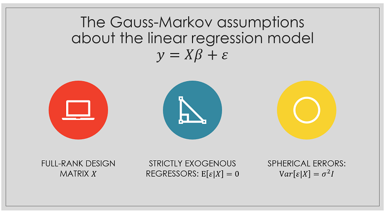
The Gauss-Markov theorem states that under certain conditions the OLS estimator is the best linear unbiased estimator (BLUE) of the vector of regression coefficients.

Conditional homoskedasticity is one of the assumptions of the Gauss-Markov theorem.

Therefore, OLS is not guaranteed to be BLUE when a regression suffers from conditional heteroskedasticity.

How to recover efficiency: the WLS/GLS estimator

The generalized least squares (GLS) estimator of the vector of regression coefficients iswhere

If all the conditions of the Gauss-Markov theorem except conditional homoskedasticity are met, OLS is not the BLUE estimator, but the GLS estimator is.

For more details and a proof, see the lecture on the generalized least squares estimator.

When is diagonal, is also called Weighted Least Squares (WLS) estimator.

Consequence for bias

Conditional heteroskedasticity does not per se introduce biases in the OLS estimator.

If conditional homoskedasticity is violated, but the other Gauss-Markov assumptions hold, then the OLS estimator remains unbiased.

Consequence for variance

When all the Gauss-Markov hypotheses hold, the conditional covariance matrix of is

When only the homoskedasticity condition is violated, then

The latter formula can be used in practice to compute the exact covariance of the OLS estimator only if:

1. is known;

2. the other assumptions of the Gauss-Markov theorem are satisfied.

Since these two conditions are unlikely to be both met in practice, we usually compute the heteroskedasticity-consistent estimator presented in the next section.

Heteroskedasticity-robust standard errors

Under fairly weak assumptions, we can prove (see here) that the asymptotic covariance matrix of iswhereis the so-called long-run covariance matrix.

In a sufficiently large sample, the covariance matrix of is approximately equal to the asymptotic one, divided by the sample size:

The matrix is consistently estimated by

If the terms of the sequence are not serially correlated, the long-run covariance matrix becomesand it is consistently estimated bywhere:

• are the residuals

• is an diagonal matrix having the squared residuals on its main diagonal.

Putting the various pieces together, we obtain

This popular estimator of the covariance matrix has various names:

• White's (1980) estimator;

• heteroskedasticity-consistent estimator (HCE);

• heteroskedasticity-robust estimator.

The square roots of the diagonal entries of the HCE matrix are estimators of the standard deviations of the regression coefficients. They are called heteroskedasticity-robust standard errors.

Condition for the consistency of White's estimator

Note that White's estimator can be used only if the terms of the sequence are uncorrelated (a condition we imposed above).

If the terms of are correlated, then we need to use another estimator called heteroskedasticity and autocorrelation consistent (HAC) or Newey-West estimator.

How to detect heteroskedasticity

There are numerous statistical tests that can be used to detect heteroskedasticity, for example:

• the Goldfeld-Quandt test;

• the Breusch-Pagan test;

• the White test.

For an introduction to these tests, you can refer, for example, to Greene (2017) and Gurajati (2017).

Models of conditional heteroskedasticity

When the linear regression is performed on time-series data, there are popular models that can be used to analyze and predict how the variance of the error terms changes through time:

• ARCH and GARCH models;

• stochastic volatility models.

More details

More mathematical details and proofs of the facts stated above can be found in the lectures on:

• the Gauss-Markov theorem;

• the generalized least squares estimator;

• the properties of the OLS estimator.

References

Greene, W.H., 2017. Econometric analysis, 8th edition, Pearson.

Gujarati, D.N., 2017. Basic econometrics, 5th edition, McGraw-Hill.

White, H., 1980. A heteroskedasticity-consistent covariance matrix estimator and a direct test for heteroskedasticity. Econometrica, 48, pp.817-838.

Keep reading the glossary

Previous entry: Factorial

Next entry: IID sequence

How to cite

Please cite as:

Taboga, Marco (2021). "Heteroskedasticity", Lectures on probability theory and mathematical statistics. Kindle Direct Publishing. Online appendix. https://www.statlect.com/glossary/heteroskedasticity.