This lecture discusses how to perform tests of hypotheses about the coefficients of a linear regression model estimated by ordinary least squares (OLS).
![]()
Table of contents
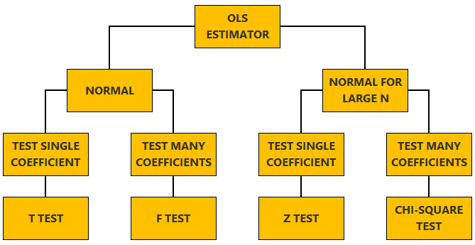
The lecture is divided in two parts:
in the first part, we discuss hypothesis testing in the normal linear regression model, in which the OLS estimator of the coefficients has a normal distribution conditional on the matrix of regressors;
in the second part, we show how to carry out hypothesis tests in linear regression analyses where the hypothesis of normality holds only in large samples (i.e., the OLS estimator can be proved to be asymptotically normal).
The regression model
is![[eq1]](data:image/gif;base64,R0lGODlhAQABAIAAANvf7wAAACH5BAEAAAAALAAAAAABAAEAAAICRAEAOw==) where:
where:
![]() is an output variable;
is an output variable;
![]() is a
is a
![]() vector of inputs;
vector of inputs;
![]() is a
is a
![]() vector of coefficients;
vector of coefficients;
![]() is an error term.
is an error term.
There are
![]() observations in the sample, so that
observations in the sample, so that
![]() .
.
We also denote:
by
![]() the
the
![]() vector of
outputs
vector of
outputs
by
![]() the
the
![]() matrix of
inputs
matrix of
inputs
by
![]() the
the
![]() vector of errors
vector of errors
Using this notation, we can
write![]()
Moreover, the OLS estimator of
![]() is
is
![]()
We assume that the design matrix
![]() has full-rank, so that the
matrix
has full-rank, so that the
matrix
![]() is invertible.
is invertible.
We now explain how to derive tests about the coefficients of the normal linear regression model.
The vector of errors
![]() is assumed to have a multivariate normal
distribution conditional on
is assumed to have a multivariate normal
distribution conditional on
![]() ,
with mean equal to
,
with mean equal to
![]() and covariance matrix equal
to
and covariance matrix equal
to![]() where
where
![]() is the
is the
![]() identity matrix and
identity matrix and
![]() is a positive constant.
is a positive constant.
It can be proved (see the lecture about the normal linear regression model) that the assumption of conditional normality implies that:
the OLS estimator
![]() is conditionally multivariate normal with mean
is conditionally multivariate normal with mean
![]() and covariance
matrix
and covariance
matrix
![]() ;
;
the adjusted sample variance of the
residualsis
an unbiased estimator of
![]() ;
furthermore, it has a
Gamma
distribution with parameters
;
furthermore, it has a
Gamma
distribution with parameters
![]() and
and
![]() ;
;
![]() is conditionally independent of
is conditionally independent of
![]() .
.
In a test of a restriction on a single coefficient, we test the
null
hypothesis![]() where
where
![]() is the
is the
![]() -th
entry of the vector of coefficients
-th
entry of the vector of coefficients
![]() and
and
![]() .
.
In other words, our null hypothesis is that the
![]() -th
coefficient is equal to a specific value.
-th
coefficient is equal to a specific value.
This hypothesis is tested with the test
statisticwhere
![]() is the
is the
![]() -th
diagonal entry of the matrix
-th
diagonal entry of the matrix
![]() .
.
The test statistic
![]() has a standard
Student's t distribution with
has a standard
Student's t distribution with
![]() degrees of freedom. For this reason, it is called a t
statistic and the test is called a t test.
degrees of freedom. For this reason, it is called a t
statistic and the test is called a t test.
Under the null hypothesis
![]() has a normal distribution with mean
has a normal distribution with mean
![]() and variance
and variance
![]() .
As a consequence, the
ratiohas
a standard normal distribution (mean
.
As a consequence, the
ratiohas
a standard normal distribution (mean
![]() and variance
and variance
![]() ).
We can
writeSince
).
We can
writeSince
![]() has a Gamma
distribution with parameters
has a Gamma
distribution with parameters
![]() and
and
![]() ,
the
ratiohas
a Gamma distribution with parameters
,
the
ratiohas
a Gamma distribution with parameters
![]() and
and
![]() .
It is also independent of
.
It is also independent of
![]() because
because
![]() is independent of
is independent of
![]() .
Therefore, the
ratiohas
a standard Student's t distribution with
.
Therefore, the
ratiohas
a standard Student's t distribution with
![]() degrees of freedom (see the lecture on the
Student's t
distribution).
degrees of freedom (see the lecture on the
Student's t
distribution).
The null hypothesis is rejected if
![]() falls outside the acceptance region.
falls outside the acceptance region.
How the acceptance region is determined depends not only on the desired size of the test, but also on whether the test is:
two-tailed
(![]() could be smaller or larger than
could be smaller or larger than
![]() ;
we do not exclude either of the two possibilities)
;
we do not exclude either of the two possibilities)
one-tailed (only one of the two things, i.e., either smaller or larger, is possible).
For more details on how to determine the acceptance region, see the glossary entry on critical values.
When testing a set of linear restrictions, we test the null
hypothesis![]() where
where
![]() is a
is a
![]() matrix and
matrix and
![]() is a
is a
![]() vector.
vector.
![]() is the number of restrictions.
is the number of restrictions.
Example
Suppose that
![]() is
is
![]() and that we want to test the hypothesis
and that we want to test the hypothesis
![]() .
We can write it in the form
.
We can write it in the form
![]() by
setting
by
setting
Example
Suppose that
![]() is
is
![]() and that we want to test whether the two restrictions
and that we want to test whether the two restrictions
![]() and
and
![]() hold simultaneously. The first restriction can be written
as
hold simultaneously. The first restriction can be written
as![]() So
we
have
So
we
have
To test the null hypothesis, we use the test
statistic![[eq28]](/images/linear-regression-hypothesis-testing__90.png) which
has an F distribution
with
which
has an F distribution
with
![]() and
and
![]() degrees of freedom. For this reason, it is called an F
statistic and the test is called an F test.
degrees of freedom. For this reason, it is called an F
statistic and the test is called an F test.
Under the null and conditional on
![]() ,
the vector
,
the vector
![]() ,
being a
linear
transformation of the normal random vector
,
being a
linear
transformation of the normal random vector
![]() ,
has a multivariate normal distribution with
mean
,
has a multivariate normal distribution with
mean![[eq29]](/images/linear-regression-hypothesis-testing__96.png) and
covariance
matrixThus,
we can
write
and
covariance
matrixThus,
we can
write![[eq31]](/images/linear-regression-hypothesis-testing__98.png) Since
Since
![]() is multivariate normal, the quadratic form
is multivariate normal, the quadratic form
![]() has a Chi-square distribution with
has a Chi-square distribution with
![]() degrees of freedom (see the lecture on
quadratic
forms involving normal vectors). Furthermore, since
degrees of freedom (see the lecture on
quadratic
forms involving normal vectors). Furthermore, since
![]() has a Gamma distribution with parameters
has a Gamma distribution with parameters
![]() and
and
![]() the
statistichas
a Chi-square distribution with
the
statistichas
a Chi-square distribution with
![]() degrees of freedom (see the lecture on the
Gamma
distribution). Thus, we can
write
degrees of freedom (see the lecture on the
Gamma
distribution). Thus, we can
write![[eq34]](/images/linear-regression-hypothesis-testing__107.png) Thus
Thus
![]() is a ratio between two Chi-square variables, each divided by its degrees of
freedom. The two variables are independent because
is a ratio between two Chi-square variables, each divided by its degrees of
freedom. The two variables are independent because
![]() depends only on
depends only on
![]() and
and
![]() depends only on
depends only on
![]() ,
and
,
and
![]() and
and
![]() are independent. As a consequence,
are independent. As a consequence,
![]() has an F distribution with
has an F distribution with
![]() and
and
![]() degrees of freedom (see the lecture on the
F distribution).
degrees of freedom (see the lecture on the
F distribution).
The F test is one-tailed.
A critical value in the right tail of the F distribution is chosen so as to achieve the desired size of the test.
Then, the null hypothesis is rejected if the F statistics is larger than the critical value.
When you use a statistical package to run a linear regression, you often get a
regression output that includes the value of an F statistic. Usually this is
obtained by performing an F test of the null hypothesis that all the
regression coefficients are equal to
![]() (except the coefficient on the intercept).
(except the coefficient on the intercept).
As we explained in the lecture on
maximum
likelihood estimation of regression models, the maximum likelihood
estimator of the vector of coefficients of a normal linear regression model is
equal to the OLS estimator
![]() .
.
As a consequence, all the usual
tests
based on maximum likelihood procedures (e.g.,
Wald,
Lagrange multiplier,
likelihood
ratio) can be employed to conduct tests of hypothesis about
![]() .
.
In this section we explain how to perform hypothesis tests about the coefficients of a linear regression model when the OLS estimator is asymptotically normal.
As we have shown in the lecture on the properties of the OLS estimator, in several cases (i.e., under different sets of assumptions) it can be proved that:
the OLS estimator
![]() is asymptotically normal, that
is,
is asymptotically normal, that
is,![]() where
where
![]() denotes convergence
in distribution (as the sample size
denotes convergence
in distribution (as the sample size
![]() tends to infinity), and
tends to infinity), and
![]() is a multivariate normal random vector with mean
is a multivariate normal random vector with mean
![]() and covariance matrix
and covariance matrix
![]() ;
the value of the
;
the value of the
![]() matrix
matrix
![]() depends on the set of assumptions made about the regression model;
depends on the set of assumptions made about the regression model;
it is possible to derive a consistent estimator
![]() of
of
![]() ,
that
is,
,
that
is,![]() where
where
![]() denotes convergence
in probability (again as
denotes convergence
in probability (again as
![]() tends to infinity). The estimator
tends to infinity). The estimator
![]() is an easily computable function of the observed inputs
is an easily computable function of the observed inputs
![]() and
outputs
and
outputs
![]() .
.
These two properties are used to derive the asymptotic distribution of the test statistics used in hypothesis testing.
In a z test the null hypothesis is a restriction on a single
coefficient:![]() where
where
![]() is the
is the
![]() -th
entry of the vector of coefficients
-th
entry of the vector of coefficients
![]() and
and
![]() .
.
The test statistic
iswhere
![]() is the
is the
![]() -th
diagonal entry of the estimator
-th
diagonal entry of the estimator
![]() of the asymptotic covariance matrix.
of the asymptotic covariance matrix.
The test statistic
![]() converges in distribution to a
standard normal
distribution as the sample size
converges in distribution to a
standard normal
distribution as the sample size
![]() increases. For this reason, it is called a z statistic
(because the letter z is often used to denote a standard normal distribution)
and the test is called a z test.
increases. For this reason, it is called a z statistic
(because the letter z is often used to denote a standard normal distribution)
and the test is called a z test.
We can write the z statistic
asBy
assumption, the numerator
![]() converges in distribution to a normal random variable
converges in distribution to a normal random variable
![]() with mean
with mean
![]() and variance
and variance
![]() .
The estimated variance
.
The estimated variance
![]() converges in probability to
converges in probability to
![]() ,
so that, by the
Continuous Mapping
theorem, the denominator
,
so that, by the
Continuous Mapping
theorem, the denominator
![]() converges in probability to
converges in probability to
![]() .
Thus, by Slutsky's theorem,
we have that
.
Thus, by Slutsky's theorem,
we have that
![]() converges in distribution to the random
variablewhich
is normal with
meanand
varianceTherefore,
the test statistic
converges in distribution to the random
variablewhich
is normal with
meanand
varianceTherefore,
the test statistic
![]() converges in distribution to
converges in distribution to
![]() ,
which is a standard normal random variable.
,
which is a standard normal random variable.
When
![]() is large, we approximate the actual distribution of
is large, we approximate the actual distribution of
![]() with its asymptotic one (standard normal).
with its asymptotic one (standard normal).
We then employ the test statistic
![]() in the usual manner: based on the desired size of the test and on the
distribution of
in the usual manner: based on the desired size of the test and on the
distribution of
![]() ,
we determine the critical value(s) and the acceptance region.
,
we determine the critical value(s) and the acceptance region.
The test can be either one-tailed or two-tailed. The same comments made for the t-test apply here.
The null hypothesis is rejected if
![]() falls outside the acceptance region.
falls outside the acceptance region.
In a Chi-square test, the null hypothesis is a set of
![]() linear
restrictions
linear
restrictions![]() where
where
![]() is a
is a
![]() matrix and
matrix and
![]() is a
is a
![]() vector.
vector.
The test statistic
is![[eq50]](/images/linear-regression-hypothesis-testing__175.png) which
converges to a
Chi-square
distribution with
which
converges to a
Chi-square
distribution with
![]() degrees of freedom. For this reason, it is called a Chi-square
statistic and the test is called a Chi-square test.
degrees of freedom. For this reason, it is called a Chi-square
statistic and the test is called a Chi-square test.
We can write the test statistic
as![[eq51]](/images/linear-regression-hypothesis-testing__177.png) By
the assumptions on the convergence of
By
the assumptions on the convergence of
![]() and
and
![]() ,
and by the Continuous Mapping theorem, we have
thatBy
Slutsky's theorem, we
have
,
and by the Continuous Mapping theorem, we have
thatBy
Slutsky's theorem, we
have![]() But
But
![]() is multivariate normal with
mean
is multivariate normal with
mean![]() and
variance
and
variance![]() Thus,
Thus,![]() but,
by
standard
results on normal quadratic forms, the quadratic form on the right hand
side has a Chi-square distribution with
but,
by
standard
results on normal quadratic forms, the quadratic form on the right hand
side has a Chi-square distribution with
![]() degrees of freedom
(
degrees of freedom
(![]() is the dimension of the vector
is the dimension of the vector
![]() )
)
When setting up the test, the actual distribution of
![]() is approximated by the asymptotic one (Chi-square).
is approximated by the asymptotic one (Chi-square).
Like the F test, also the Chi-square test is usually one-tailed.
The desired size of the test is achieved by appropriately choosing a critical value in the right tail of the Chi-square distribution.
The null is rejected if the Chi-square statistics is larger than the critical value.
Want to learn more about regression analysis? Here are some suggestions:
Please cite as:
Taboga, Marco (2021). "Linear regression - Hypothesis testing", Lectures on probability theory and mathematical statistics. Kindle Direct Publishing. Online appendix. https://www.statlect.com/fundamentals-of-statistics/linear-regression-hypothesis-testing.
Most of the learning materials found on this website are now available in a traditional textbook format.